Hello again! With the help of my friend Ben, another Jane Street puzzle has been solved. Today, I will walk you through our solution.

This puzzle was more mathematical than last month. It involved calculating the probability that a randomly generated circle, within a 1x1 square, lies outside the square. This circle has a diameter determined by two points that are uniformly generated within the square.

Of course a simulator was the natural first step. This would allow us to know if we were close to the actual solution.

Here is the code:

import random
import math

num_trials = 10000000
num_success = 0

for i in range(num_trials):
    x1 = random.random()
    y1 = random.random()
    x2 = random.random()
    y2 = random.random()
    sum_x = x1 + x2 
    sum_y = y1 + y2
    dist = math.sqrt((x2 - x1)**2 + (y2 - y1)**2)
    cond_1 = sum_x + dist > 2
    cond_2 = sum_x - dist < 0
    cond_3 = sum_y + dist > 2
    cond_4 = sum_y - dist < 0
    if cond_1 or cond_2 or cond_3 or cond_4:
        num_success += 1

print(num_success / num_trials)

This probability ended up being around ~0.4764. At least we knew an approximate solution. The hard part was we needed the closed form solution.

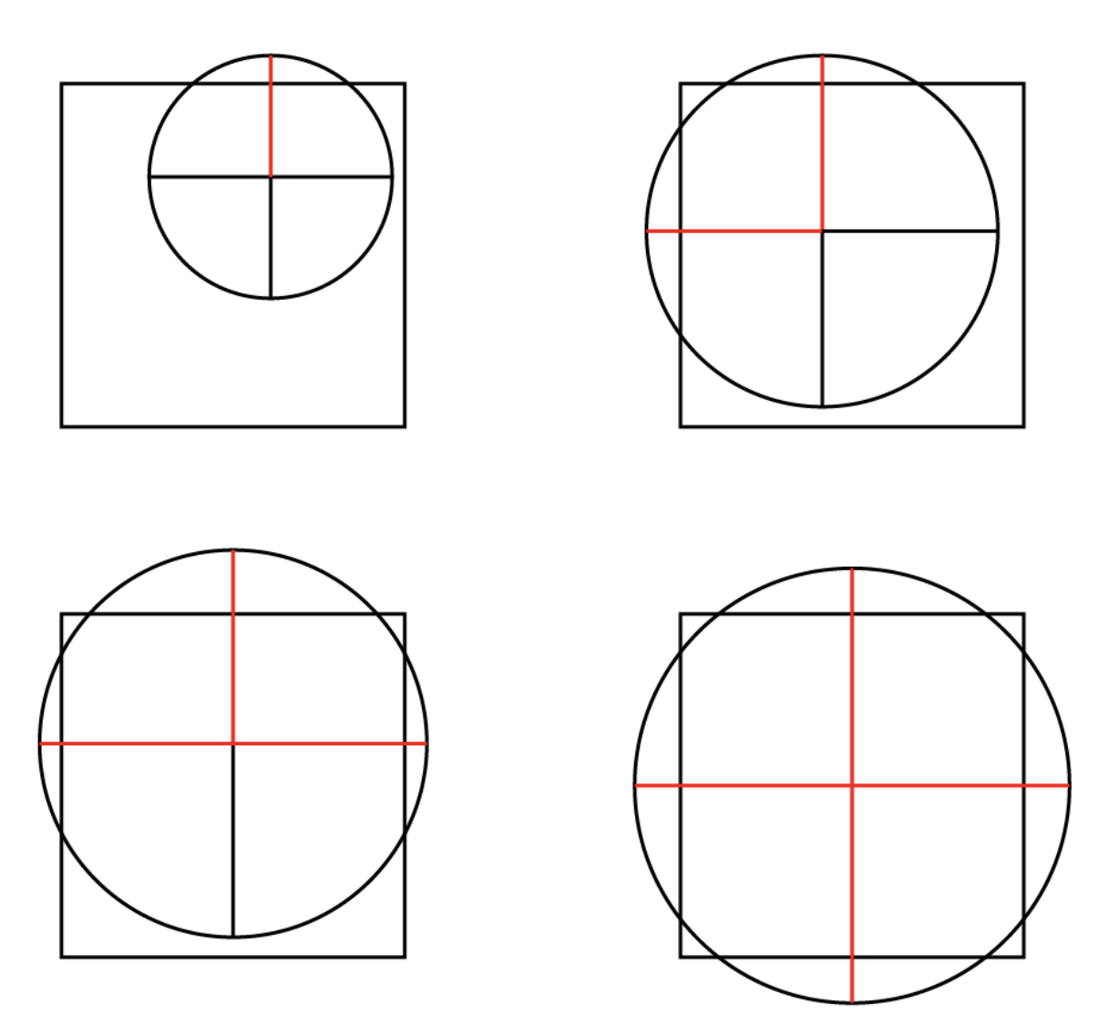
We first attempted to find the probability that one of the four points of the circle broke the outside of the square. This led to many edge cases, though, which became hard to deal with. As you can see from the picture below, the circle could potentially break two, three, or all four sides of the square. Calculating the probability of all of these events happening quickly became too complex.

So, naturally the complement became our new hope. We had come up with a couple equations that modeled these four points that could help us determine if the circle was outside of the square. They all looked like this:

Where (x1, y1) and (x2, y2) were the uniform random points selected within the square.

Naturally, we had already thought of convolving these uniform random variables and then integrating over the PDF to find the probability that this number was within a bound. This equation, representing the right point, would be bounded below one.

Finding this probability was a struggle, but with the help of Mathematica it was greatly simplified. Here is the Mathematica code:

1 - CDF[TransformedDistribution[
   x1 + x2 +
    Sqrt[(x1 - x2)^2 + (y1 - y2)^2], {Distributed[x1,
     UniformDistribution[{0, 1}]],
    Distributed[x2, UniformDistribution[{0, 1}]],
    Distributed[y1, UniformDistribution[{0, 1}]],
    Distributed[y2, UniformDistribution[{0, 1}]]}], 2]

Which evaluated to

Now, assuming every point is independently within its bound, the answer would theoretically be

Which was SOOO close to the simulated answer! Just 0.03 away. Ben assured me that it cannot be right due to the non-independence of the four points breaking the square. So, we had to try something else.

After a day of minimal progress, I had a (potentially) breakthrough idea. What if…

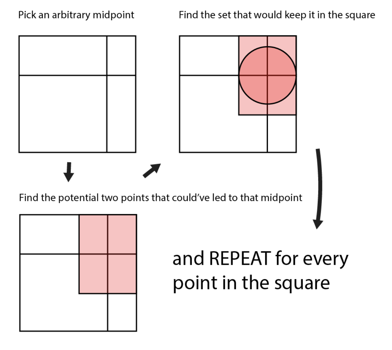
But we couldn’t just integrate and repeat the same thing for every midpoint in the square. This solution depended on knowing the radius of that circle region of midpoints that would not break the outside of the square, which equaled the distance to the closest side of the square. Therefore, the integration would have to be broken into four parts:

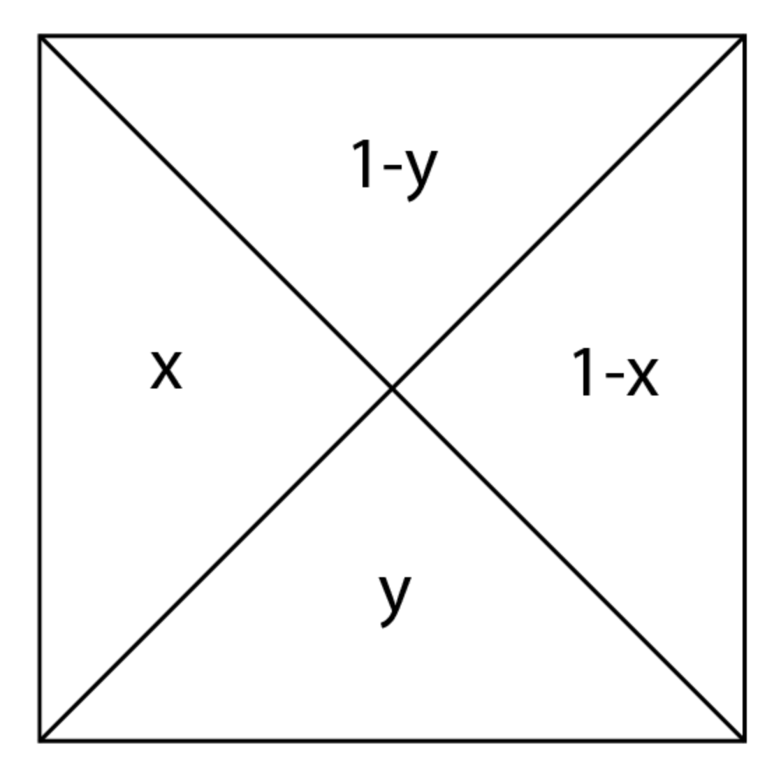
Where the letter inside each region represents the distance to the closest side. Unfortunately, this was not enough. We needed to split up the square into 8 regions due to the fact that the dimensions of the rectangle that represented all possible points would change depending on what quarter of the square the midpoint was on. So, we had this:

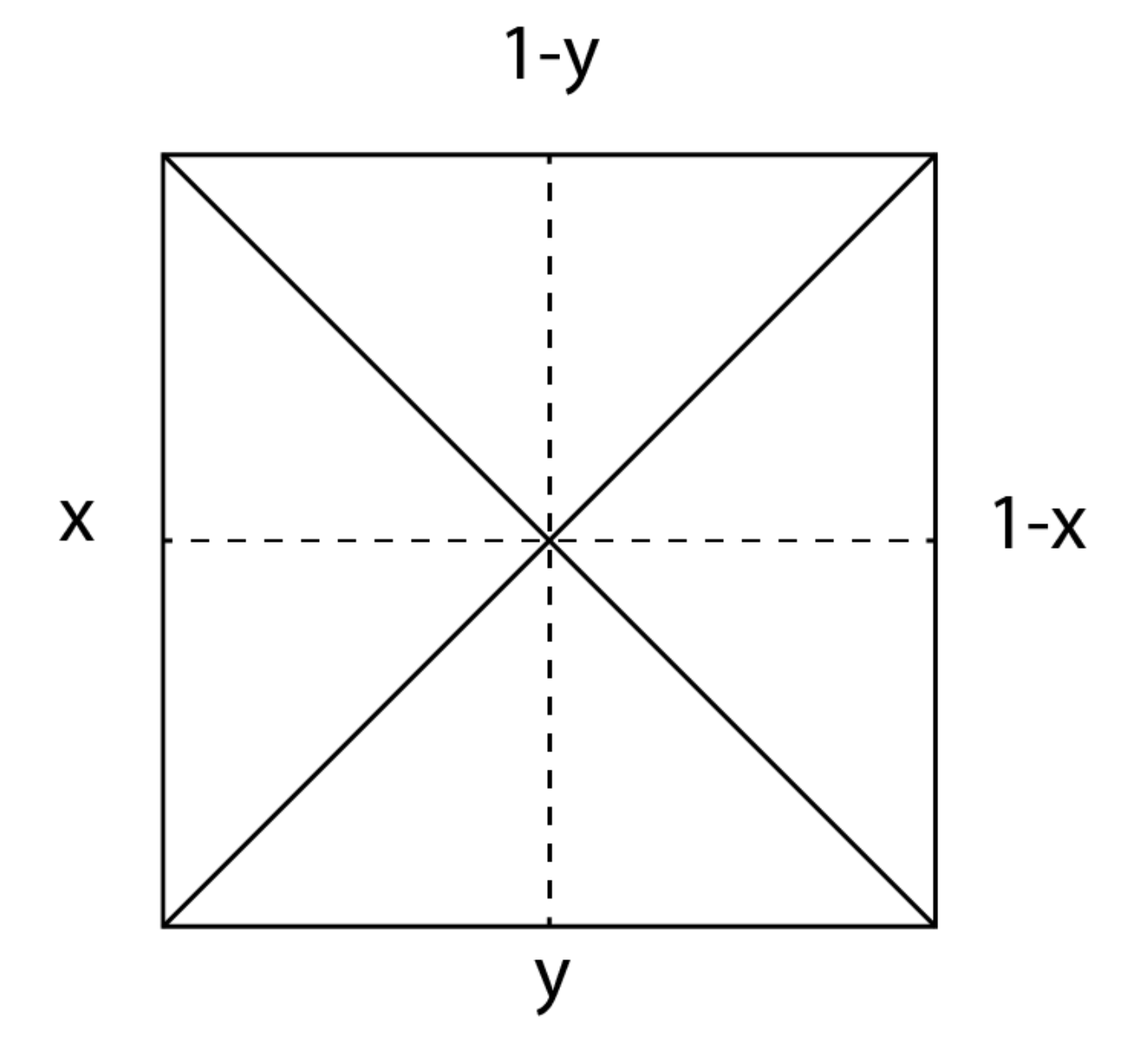
This allowed us to set up the integral:

Where the integrand represents the probability that the midpoints lie outside the circle mentioned above. The problem is, this only represented the probability that the two points constructing the midpoint were outside the circle. It doesn’t compute the compound probability that the midpoint is even where it is. To do this, we estimated what the probability distribution for each midpoint looks like, which ended up being just x and y for the bottom left quadrant. Multiplying them and putting them in the integrand, the integral now looks like:

Naturally, we decided to multiply the result by 128, which seemed natural given the potential symmetries in this problem. This gave us:

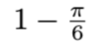
Which seemed to match with the simulation. It happened to be right!

Thanks for reading!